What is Aggregate Supply?

Aggregate supply, also known as domestic final supply, is the total supply of goods and services available for sale in a country's economy at a specific time. 

Firms make decisions about what quantity to supply based on the profits they expect to earn. They determine profits, in turn, by the price of the outputs they sell and by the prices of the inputs, like labor or raw materials, that they need to buy. 

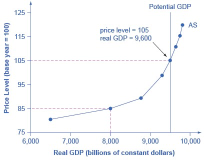
Aggregate supply (AS) refers to the total quantity of output (i.e. real GDP) firms will produce and sell. 

The aggregate supply (AS) curve shows the total quantity of output (i.e. real GDP) that firms will produce and sell at each price level.

Aggregate supply (AS) slopes up, because as the price level for outputs rises, with the price of inputs remaining fixed, firms have an incentive to produce more to earn higher profits. The potential GDP line shows the maximum that the economy can produce with full employment of workers and physical capital.

The diagram's horizontal axis shows real GDP—that is, the level of GDP adjusted for inflation. The vertical axis shows the price level, which measures the average price of all goods and services produced in the economy. 

In other words, the price level in the AD-AS model is a depiction of the GDP Deflator. 

Remember that the price level is different from the inflation rate. Visualize the price level as an index number, like the Consumer Price Index, while the inflation rate is the percentage change in the price level over time.

As the price level rises, real GDP rises as well. 

The price level on the vertical axis represents prices for final goods or outputs bought in the economy—i.e. the GDP deflator—not the price level for intermediate goods and services that are inputs to production.

 Thus, the AS curve describes how suppliers will react to a higher price level for final outputs of goods and services, while holding the prices of inputs like labor and energy constant. If firms across the economy face a situation where the price level of what they produce and sell is rising, but their costs of production are not rising, then the lure of higher profits will induce them to expand production. In other words, an aggregate supply curve shows how producers as a group will respond to an increase in aggregate demand.

Shifts in Aggregate Supply or Aggregate Demand

The original equilibrium in the AD/AS diagram will shift to a new equilibrium if the AS or AD curve shifts. When the aggregate supply curve shifts to the right, then at every price level, producers supply a greater quantity of real GDP. When the AS curve shifts to the left, then at every price level, producers supply a lower quantity of real GDP. This module discusses two of the most important factors that can lead to shifts in the AS curve: productivity growth and changes in input prices.

Productivity and Shifts in the Aggregate Supply Curve

In the long run, the most important factor shifting the AS curve is productivity growth. Productivity means how much output can be produced with a given quantity of labor. One measure of this is output per worker or GDP per capita. Over time, productivity grows so that the same quantity of labor can produce more output. 

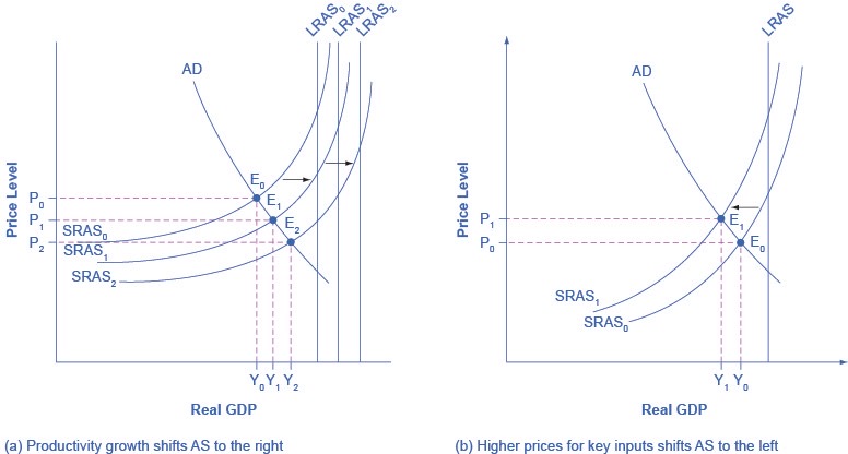
A higher level of productivity shifts the AS curve to the right, because with improved productivity, firms can produce a greater quantity of output at every price level.

The rise in productivity causes the SRAS curve to shift to the right. The original equilibrium E₀ is at the intersection of AD and SRAS₀. When SRAS shifts right, then the new equilibrium E₁ is at the intersection of AD and SRAS₁, and then yet another equilibrium, E₂, is at the intersection of AD and SRAS₂.

Shifts in SRAS to the right, lead to a greater level of output and to downward pressure on the price level. (b) A higher price for inputs means that at any given price level for outputs, a lower real GDP will be produced so aggregate supply will shift to the left from SRAS₀ to SRAS₁. The new equilibrium, E₁, has a reduced quantity of output and a higher price level than the original equilibrium (E₀).

A shift in the SRAS curve to the right will result in a greater real GDP and downward pressure on the price level, if aggregate demand remains unchanged. However, if this shift in SRAS results from gains in productivity growth, which we typically measure in terms of a few percentage points per year, the effect will be relatively small over a few months or even a couple of years. 

Changes in Input Prices Shift the Aggregate Supply Curve

Higher prices for inputs that are widely used across the entire economy can have a macroeconomic impact on aggregate supply. Examples of such widely used inputs include labor and energy products. Increases in the price of such inputs will cause the SRAS curve to shift to the left, which means that at each given price level for outputs, a higher price for inputs will discourage production because it will reduce the possibilities for earning profits.

Conversely, a decline in the price of a key input like oil will shift the SRAS curve to the right, providing an incentive for more to be produced at every given price level for outputs.

Other Factors Causing a Shift in the SRAS Curve?

Along with energy prices, two other key inputs that may shift the SRAS curve are the cost of labor, or wages, and the cost of imported goods that we use as inputs for other products. In these cases as well, the lesson is that lower prices for inputs cause SRAS to shift to the right, while higher prices cause it to shift back to the left. Note that, unlike changes in productivity, changes in input prices do not generally cause LRAS to shift, only SRAS.

The aggregate supply curve can also shift due to shocks to input goods or labor. For example, an unexpected early freeze could destroy a large number of agricultural crops, a shock that would shift the AS curve to the left since there would be fewer agricultural products available at any given price.

Similarly, shocks to the labor market can affect aggregate supply. An extreme example might be an overseas war that required a large number of workers to cease their ordinary production in order to go fight for their country. In this case, SRAS and LRAS would both shift to the left because there would be fewer workers available to produce goods at any given price.

Related Topics

• Supply-Side Economics
• Say's Law
• Laffer Curve
• Neo-Classical Economics
• New Keynesian Economics
• Classical Economics
• Supply-Side Economics
• Keynesian Economics
• Keynes' Law
• Keynesian Analysis
• Demand Side Theory
• Market Forces
• Aggregate demand
  
• Aggregate Demand Curve (and shifts)
• Aggregate supply
• Aggregate Supply Curve (and Shifts)
• Aggregate Demand / Aggregate Supply Models
• Potential GDP
• Aggregate Supply and Demand Equilibrium
• Aggregate Supply and Aggregate Demand in Macroeconomics and Microeconomics
• Input-Output Model
• Stagflation
• Growth and Recessions in the Aggregate Demand - Aggregate Supply Model
• Unemployment in the Aggregate Demand - Aggregate Supply Model
• Inflation in the Aggregate Demand - Aggregate Supply Model
• Keynesian, Intermediate, and Neoclassical Zones