What is Aggregate Demand?

Aggregate demand is a macroeconomic term that refers to the total demand or exchange for products at a particular time and at a stated price. It is the total amount of goods and services produced in an economy, and the total demand for each commodity. Aggregate demand does not measure the standard of living in a nation (unlike demand in microeconomics), but rather it focuses on the demand at a given period and price.

What Makes Up Aggregate Demand?

Aggregate demand is equivalent to the gross domestic product (GDP) of an economy as each focuses on the total demand for commodities at different price values. Both terms share the same market pattern and would move in the same position in terms of accounting. It is, however, important to note that the aggregate demand is only equivalent to the GDP in the long run as it is only at this point that it adjusts to the price level of commodities in the market. This is due to the fact that short-run production is primarily focused on getting equilibrium demand for a single price and not for potential market prices in the future. For simplicity, price value is said to be 1. There are also other errors involved in calculating aggregate demand as it isnt specific and works with a general model even for distinct products. As long as commodities are supplied and demanded at the same price level, they are said to be equals, even without considering whether they are corporate, consumer or national commodities.

Mathematical Solution for Aggregate Demand

In calculating aggregate demand, one must employ the method used for computing an economys GDP, which in this case is the Keynesian equation. Using this equation, we have that: AD= C + I + Nx Where; A = Aggregate Demand C = Consumer spending on commodities I = Personal Investments and corporate financing G = Government spending (National budgets and the likes) Nx = Net export (the remains after imports have been removed).

Explaining Aggregate Demand with Assumptions

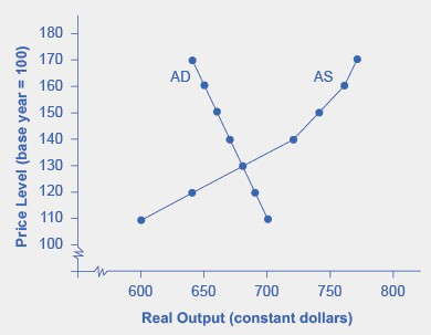
In a graphical illustration or representation of aggregate demand, the total output (mostly known as quantity on curves) goes on the X-axis, and the Overall Price level of all commodities goes on the Y-axis. Since aggregate demand is a type of demand, the curve typically slopes downward from left to right, thus portraying the market demand in relation to price. Here, if the price of commodities were to increase to its highest, the curve would be at the top left, signifying that fewer purchases are made. When the price drops to its lowest, the curve reaches the far right, signifying that demand has increased much more than before. The curve is also affected by tax rates as more expenses reduce taxes.

Determinants of Aggregate Demand

Given below are some factors which influence aggregate demand:

• Foreign Exchange rate change: Foreign Exchange (also called Forex or Currency Exchange) affects the aggregate demand of an economy. For instance, if the Canadian dollar were to incur a drop, the value of imported goods will become costlier, while the price of products manufactured in the nation will become cheaper. The opposite happens if the CAD were to increase.
• Personal Income: It goes without saying that the richer a person gets, the more hed want to satisfy his wants.
• Personal Opinions about Fluctuation: If a person who purchases air conditioners for $400 each believes that the price will increase to $450 each in the near future, he or she will try to purchase and store as much air conditioners as possible at the current rate of $400, and this causes an increase in aggregate demand. On the other hand, if that individual feels that the price would drop to $350 in the near future, he or she might choose to wait till that time, thus causing a drop in the aggregate demand.
• Shift in Real Interest rates: This mostly applies to capital goods. The real interest rate determines consumers behavior in making purchases. The higher the rate, the higher the cost of commodities, and the lower the demand. Also, the lower the rates, the lower the cost of commodities, and the higher the demand.

Controversies Surrounding Aggregate Demand

An increase in aggregate demand secures an increase in the GDP of an economy but doesnt actually certify economic growth. Both concepts make use of the same equation, which is the Keynesian equation in this case, which analyses only the growth but discards the cause. In economics, knowing why something exists in an economy is vital, but this is nowhere to be found in the relationship between aggregate demand and GDP. This issue has raised up different controversies. According to 18th Century French economist, Jean-Baptiste Say, consumption is as a result of production, and it is mostly dependent on it. He goes on to propose what is known today as Says Law, a theory that states that social wants are limitless, and only held in check by what can be produced. For example, people with enough money to purchase 200 units of canned tunas will be forced to buy less if only 20 units are available. This realistic example shows that production is a barrier to want. However, using the demand-and-supply model, one can see that Jean-Baptistes statement does not entirely hold. According to British economist John Maynard Keynes, supply is as a result of demand, as the more consumers place an order for a particular item, the more it would be produced. This theory came to be referred to as the Keynesian Theory, and it gathered a large number of followers. According to this theory, on the demand-side of economics, the demand for a product drives production as well as the money which consumers are willing to spend on that product. So if people are willing to pay $40 per can of tuna instead of $30, it is only natural to see large bulk of cans being tossed into the market daily. Keynes also stated that unemployment in an economy is as a result of inefficient aggregate demand, as the more the demand for an item, the more workers will be needed in the production and distribution of that particular item. He further proposed that government spending could influence employment by creating infrastructures that would allow displaced workers and resources to be redeployed. These two theorists have gained a huge following, with the Austrian School and real business cycle adhering to the teachings of Says Law. They argue that consumption is only possible after production, stating that an increase in production stirs an increase in consumption and not the other way around. They further imply that increasing spending rather than production will cause a shift in prices and would be deemed a misuse of wealth. Followers of Keynes Theory, however, believe that the consumers can lay waste to products that are manufactured by deciding to hoard their wealth and not make purchases. Another school of thoughts, however, believe that this wouldnt affect production but rather reduce prices to the point that it makes the rational producer have second thoughts about supplying more products. They further argue that hoarded money does not necessarily disappear as consumers will surely have something to spend them on.

Shortcomings of Aggregate Demand

In macroeconomics, aggregate demand measures different transactions of various individuals in millions for several reasons. This poses some difficulties in analyzing variations, regression or efficiently examining casualty as well as collinearity. This is popularly term aggregation problem or ecological inference fallacy in statistics.

Aggregate Demand Curve

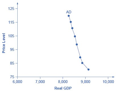
The aggregate demand (AD) curve shows the total spending on domestic goods and services at each price level.

Just like the aggregate supply curve, the horizontal axis shows real GDP and the vertical axis shows the price level. The AD curve slopes down, which means that increases in the price level of outputs lead to a lower quantity of total spending. The reasons behind this shape are related to how changes in the price level affect the different components of aggregate demand. The following components comprise aggregate demand: consumption spending (C), investment spending (I), government spending (G), and spending on exports (X) minus imports (M): C + I + G + X – M.

Aggregate demand (AD) slopes down, showing that, as the price level rises, the amount of total spending on domestic goods and services declines.

The wealth effect holds that as the price level increases, the buying power of savings that people have stored up in bank accounts and other assets will diminish, eaten away to some extent by inflation. Because a rise in the price level reduces people’s wealth, consumption spending will fall as the price level rises.

The interest rate effect is that as prices for outputs rise, the same purchases will take more money or credit to accomplish. This additional demand for money and credit will push interest rates higher. In turn, higher interest rates will reduce borrowing by businesses for investment purposes and reduce borrowing by households for homes and cars—thus reducing consumption and investment spending.

The foreign price effect points out that if prices rise in the United States while remaining fixed in other countries, then goods in the United States will be relatively more expensive compared to goods in the rest of the world. U.S. exports will be relatively more expensive, and the quantity of exports sold will fall. U.S. imports from abroad will be relatively cheaper, so the quantity of imports will rise. Thus, a higher domestic price level, relative to price levels in other countries, will reduce net export expenditures.

Among economists all three of these effects are controversial, in part because they do not seem to be very large. For this reason, the aggregate demand curve slopes downward fairly steeply. The steep slope indicates that a higher price level for final outputs reduces aggregate demand for all three of these reasons, but that the change in the quantity of aggregate demand as a result of changes in price level is not very large.

Changes in Consumption Affect Aggregate Demand

When consumers feel more confident about the future of the economy, they tend to consume more. If business confidence is high, then firms tend to spend more on investment, believing that the future payoff from that investment will be substantial. Conversely, if consumer or business confidence drops, then consumption and investment spending decline.

The Organization for Economic Development and Cooperation (OECD) publishes one measure of business confidence: the "business tendency surveys". The OECD collects business opinion survey data for 21 countries on future selling prices and employment, among other business climate elements. After sharply declining during the Great Recession, the measure has risen above zero again and is back to long-term averages (the indicator dips below zero when business outlook is weaker than usual). Of course, either of these survey measures is not very precise. They can however, suggest when confidence is rising or falling, as well as when it is relatively high or low compared to the past.

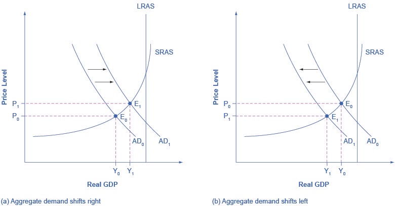
Because economists associate a rise in confidence with higher consumption and investment demand, it will lead to an outward shift in the AD curve, and a move of the equilibrium, from E₀ to E₁, to a higher quantity of output and a higher price level.

Consumer and business confidence often reflect macroeconomic realities; for example, confidence is usually high when the economy is growing briskly and low during a recession. However, economic confidence can sometimes rise or fall for reasons that do not have a close connection to the immediate economy, like a risk of war, election results, foreign policy events, or a pessimistic prediction about the future by a prominent public figure. U.S. presidents, for example, must be careful in their public pronouncements about the economy. If they offer economic pessimism, they risk provoking a decline in confidence that reduces consumption and investment and shifts AD to the left, and in a self-fulfilling prophecy, contributes to causing the recession that the president warned against in the first place. 

The below figure shows a shift of AD to the left, and the corresponding movement of the equilibrium, from E₀ to E₁, to a lower quantity of output and a lower price level.

(a) An increase in consumer confidence or business confidence can shift AD to the right, from AD₀ to AD₁. When AD shifts to the right, the new equilibrium (E₁) will have a higher quantity of output and also a higher price level compared with the original equilibrium (E₀). In this example, the new equilibrium (E₁) is also closer to potential GDP. An increase in government spending or a cut in taxes that leads to a rise in consumer spending can also shift AD to the right. (b) A decrease in consumer confidence or business confidence can shift AD to the left, from AD₀ to AD₁. When AD shifts to the left, the new equilibrium (E₁) will have a lower quantity of output and also a lower price level compared with the original equilibrium (E₀). In this example, the new equilibrium (E₁) is also farther below potential GDP. A decrease in government spending or higher taxes that leads to a fall in consumer spending can also shift AD to the left.

Government Choices Shift Aggregate Demand

Government spending is one component of AD. Thus, higher government spending will cause AD to shift to the right, while lower government spending will cause AD to shift to the left. 

Tax policy can affect consumption and investment spending, too. Tax cuts for individuals will tend to increase consumption demand, while tax increases will tend to diminish it. Tax policy can also pump up investment demand by offering lower tax rates for corporations or tax reductions that benefit specific kinds of investment. Shifting C or I will shift the AD curve as a whole.

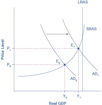
During a recession, when unemployment is high and many businesses are suffering low profits or even losses.

The original equilibrium during a recession is at point E₀, relatively far from the full employment level of output. The tax cut, by increasing consumption, shifts the AD curve to the right. At the new equilibrium (E₁), real GDP rises and unemployment falls and, because in this diagram the economy has not yet reached its potential or full employment level of GDP, any rise in the price level remains muted. Read the following Clear It Up feature to consider the question of whether economists favor tax cuts or oppose them.

Whether the economy is in a recession is illustrated in the AD/AS model by how close the equilibrium is to the potential GDP line as indicated by the vertical LRAS line. In this example, the level of output Y₀ at the equilibrium E₀ is relatively far from the potential GDP line, so it can represent an economy in recession, well below the full employment level of GDP. In contrast, the level of output Y₁ at the equilibrium E₁ is relatively close to potential GDP, and so it would represent an economy with a lower unemployment rate.

Government spending and tax rate changes can be useful tools to affect aggregate demand. Other policy tools can shift the aggregate demand curve as well. For example, the Federal Reserve can affect interest rates and credit availability. Higher interest rates tend to discourage borrowing and thus reduce both household spending on big- ticket items like houses and cars and investment spending by business. Conversely, lower interest rates will stimulate consumption and investment demand. Interest rates can also affect exchange rates, which in turn will have effects on the export and import components of aggregate demand.

Here, the key lesson is that a shift of the aggregate demand curve to the right leads to a greater real GDP and to upward pressure on the price level. Conversely, a shift of aggregate demand to the left leads to a lower real GDP and a lower price level. Whether these changes in output and price level are relatively large or relatively small, and how the change in equilibrium relates to potential GDP, depends on whether the shift in the AD curve is happening in the AS curve's relatively flat or relatively steep portion.

Related Topics

• Supply-Side Economics
• Say's Law
• Laffer Curve
• Neo-Classical Economics
• New Keynesian Economics
• Classical Economics
• Supply-Side Economics
• Keynesian Economics
• Keynes' Law
• Keynesian Analysis
• Demand Side Theory
• Market Forces
• Aggregate demand
  
• Aggregate Demand Curve (and shifts)
• Aggregate supply
• Aggregate Supply Curve (and Shifts)
• Aggregate Demand / Aggregate Supply Models
• Potential GDP
• Aggregate Supply and Demand Equilibrium
• Aggregate Supply and Aggregate Demand in Macroeconomics and Microeconomics
• Input-Output Model
• Stagflation
• Growth and Recessions in the Aggregate Demand - Aggregate Supply Model
• Unemployment in the Aggregate Demand - Aggregate Supply Model
• Inflation in the Aggregate Demand - Aggregate Supply Model
• Keynesian, Intermediate, and Neoclassical Zones